How to create a unique target chart in Excel

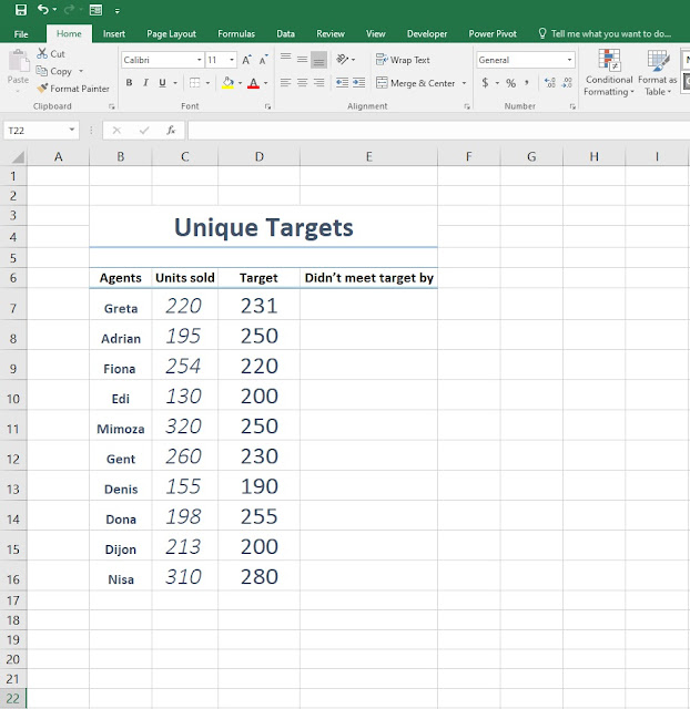
Hello everyone, and welcome back to another tutorial where this time we're going to create a unique target chart using Microsoft Excel. If you've followed the previous posts you will get the idea on what we will try to do and shouldn't have any difficulties whatsoever. 1. First step, fill in the cells with the information given bellow. Once we're finished with this tutorial you can create the table based on your needs and preferences. 2. Step two, by now you probably noticed the headers consisting the Agents, Units sold, Target and Didn't meet target by. What you will do now is under the Didn't meet target by cell type the formula =MAX(D7-C7,0) in order to avoid the IF function we've added MAX instead, where we set 0 as our number limit so we don't have net results like -12, -25, -36 etc. 3. Step three, we've added another header Target overachieved where we will type the formula...