How to create a student result sheet in Excel
In this tutorial I'm going to show you how to use the IF function (logical test) with the True or False value. Also, how to use symbols in excel.
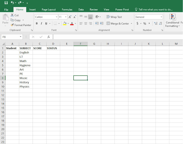
1. For us to use the IF function and Tick symbols, firstly we have to create a basic student data sheet where you can type the necessary information such as: Student name, subject, score, status etc. The first step for you to do is write down a simple student sheet with the as seen on the picture below.
2. Step two, on the Student column select the cells from A2 to A10, right click > format cells click on the merge cells box, then set the orientation to 90 degrees and click OK.
3. Once you've merged the cells, write down the name of your student and make sure to align your content and text to center and middle as seen on the picture below. Also, make sure you change your font size to your liking as well.
4. Next step, write down the scores of your student on each of the subjects.
5. Now the critical step towards this tutorial is for you to write a logical IF function with a True or False value. And how can we do that? Simply, make sure you set the output on the D2 cell so the formula will take effect in order. Next, write down this formula: =If(C2>=75,"PASSED","FAILED")
What we did with this formula is that we used an IF function to determine a logical outcome depending on the information we provided on the table. Next, we open the parentheses and we select or write down the C2 cell that contains the score on each of the subjects. What we do next is we've set the criteria to greater or equal than 75 (>=75). Once we put a comma we already told the computer, in this case the IF function what to do. Now we continue by setting the True or False value. Take note that the True value always comes first, so we open and close the True value with a double apostrophe, " " . In this case what we want as a True value is a PASSED outcome if the exam score is 75 or higher. Once again to move to the next step, we use a comma for that and we start using the double apostrophes for the FALSE value as well where inside the double apostrophe we write FAILED as our outcome if the score is 74 or lower. Finally we close the parentheses, click enter and we are all set.
6. Once you've pressed enter you should have a PASSED or FAILED outcome on your student status. To do the same for the rest of the subjects, simply drag and drop from the D2 cell in order to get an automatic result based on the formula we've just put. Note that now you can change your subject scores and the formula will take care of the rest whether the student has passed or failed the exam based on the criteria we've set, which is (C2>=75).
7. Now that the table or student data sheet is complete, it's time for us to put and format the tick symbol, on the score column. To do that, head over to Conditional Formatting > New Rule.
8. Once the new formatting rule window opens, there is a series of changes that you have to make. Firstly, click on the Format Style and set it to Icon Sets. Next, click on the Icon Style and select the Tick symbol. Under the Icon category, change the ticks that you want to be shown on the column, also on the third symbol category set it to No Cell Icon. Finally, under Value set it to 75 and 0 as seen on the picture below and don't forget under Type, set it to Number for both categories. Click OK and the symbols will appear.
9. Now that the student data sheet is complete you can add a bit of a design element depending on your liking. What I've done is selected a header design and under Borders > Draw Border I've manually drawn borders on the side of the data sheet to give it a more complete look.
Here's an idea on what the table or student data sheet will look like once we've done all of the steps mentioned above.
10. It's not necessary, however, you can always convert your student data sheet into a table. By doing so, you're going to have a much wider access to your student data base, as you can see on the picture below, you can select a particular, subject, score or status to be shown on your table.
11. If you wish to add more students to your data sheet, you can either drag and drop the table for extension, or for a more precise solution simply, copy and paste the subject column just under the data sheet. Format and merge the cells on the student column and write down the name of your next student.
Hopefully, by now you have a clear indication on how to create a student data sheet so you can start from the beginning and create one for yourself depending on your needs and priorities.
Here's also a video showcase of this tutorial.


Comments
Post a Comment