How to use math formulas in Excel

Welcome to another tutorial today where we're going to learn how to use simple and basic math formulas in Excel. With a step by step guide we will go through some basic math formulas and how to use them in your day to day life using Microsoft Excel.

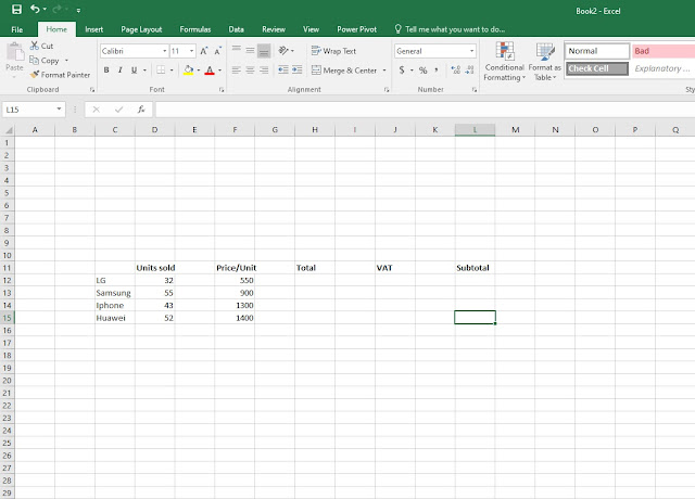
   1. Before we start using the math formulas, firstly, I've created a field of useful information as my input that is going to help you orientate on where and when you should use the formulas. As you can see from the picture below, I've created a simple sales table representing the number of smart phones sold. So, open a blank workbook and write down the necessary information as in the picture below.

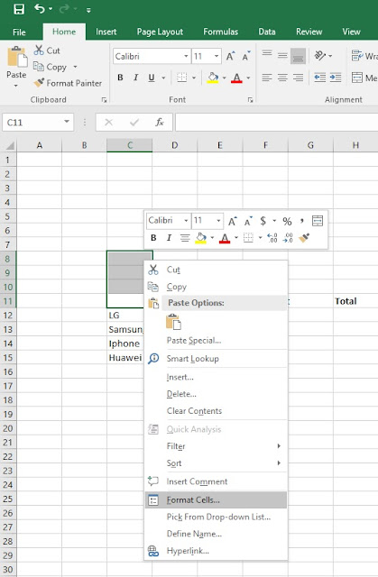
   2. Once you've wrote down all the information, you'll notice that the column just above the manufacturer brand is empty, that's because the column is not wide enough to fit large words. In order to make that word completely visible you could either reduce the font size, widen the column or in my case you can format the columns so that the entire word can fit in one column. First step, select a couple of columns above (depending on the word) Right click > Format Cells. 

   3. Once you've clicked on Format Cells, a small window will appear as seen on the picture below showing a number of options on how to format the cells. The first step here is for you to check Merge Cells under the Text control category. Secondly, on the right side of the window under Orientation drag the clock shaped arrow icon and place it diagonally depending on your needs. In my case, I've tilted the word in a 62 degree shape. Finally, once you're done, click OK.

This is what would look like once we click OK.

   4. For further formatting of the cells, select the columns under Price/Unit > Right click > Format Cells and a window will appear where you can change the formatting of the cells depending on your liking or priorities. Under the Category, you have various formatting options. In my case I've selected Currency because under the Price/Unit column we have numbers representing the amount of money sold per unit. Moreover, I've set the Decimal place to 0 and under Symbol, $.  Finally, click OK and everything will be set.

   5. Now that everything is at it's place, we can finally start typing the math formulas. Before we start typing, if you go under Formulas, and as seen on the picture below just inside the red rectangle there you can find different formulas and functions to suit your needs, whereas, just under the red rectangle, there's a formula bar and that's where the formulas are written. Also, important to note that in Excel whenever you want to write a formula you should always start the formula with =

   6. This is where the fun starts using the math formulas. Just so you remember, you can either write the formula in the formula bar, or in the cell that you've selected. However, before you write down the formula, you have to select a cell as an output.  Also note that once you chose the cell you wish to write down the formula, it will automatically display the formula that you're writing on the formula bar. In my case I've selected the H12 cell as an output and what I want to do is multiply the D12 and F12 cell where the output is going to be on the H12 cell as mentioned before. And how do you multiply the cells? Simply write down this multiplying formula =D12*F12 and press enter and you'll have the cells calculated by the computer. 

   7. If you wish to manually write down the formulas you can simply just selec the cells you want to multiply for example: =D13*F13, =D14*F14 and so on. However, there is a quick and simple way for you to calculate the remaining cells. If you look closely just under the Total, we already have placed the formula and if we click on that cell, on the bottom right of the green rectangle there is a small rectangle shape where you can drag and drop down until you wish to calculate the cells. Once you release the mouse click, the cells will be calculated automatically, without having the need to write down the formulas manually.   

   8. For the next step, we're going to calculate the VAT of the sold units/products. Select the output on J12, just under the VAT and write this formula: =H12*18% . This formula is going to calculate the 18% of the VAT. Of course, you can set the % any number you like, for a simplified tutorial I've used a common 18% VAT. Once you click enter you should have the result, also make sure you drag and drop the cell for an automatic calculation. 

   9. By now you should have a clear indication on how this table is evolving and what sort of formulas we are using. The final step to complete this sales table is for you to select the output on the L12 and start writing the formula: =H12-J12 what this formula is going to do is subtract the VAT cost from the Total income. Click enter and drag and drop for automatic calculation of the cells.

Here is couple of simple and basic math formulas for you to use in Excel:

=A1+B1

=A1-B1

=A1*B1

=A1/B1

=A1*(insert number) %

   10. Now that we have the sales table completed you can use Conditional Formatting for adding some design elements to your table. To do that, select the cells or columns you wish to tweak with a bit of visual design, and go Home > Conditional Formatting > Data Bars. And select your favorite formatting depending on your requirements. Of course, you can choose different formatting under the Conditional Formatting > category.

You can play around the Conditional formatting > category, as I did (see picture below) until you find what you need. On each column, I used a different formatting just so you have a clear indication on how to use the formatting tool.

Here's also a video showcase on how to use math formulas in Excel.