How to create a simple student data entry in Excel
Here's a very easy and simple student data entry tutorial that I'm going to show you how to do it in very easy steps. Once you get around this tutorial you can create one for yourself using different categories, depends how it suits your best needs. So, let's get started!
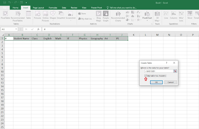
1. First step, write down the categories as seen on the picture below, select all the cells > insert table > My table has headers > OK.
2. Step two, once you've created the table go to File > Options.
3. Step three, once you click options, a window under the name excel options is going to appear where we have to enable the data entry form command.
- Click the Quick Access Toolbar and under Choose commands form select Commands not in ribbon.
- Scroll down until you find Form, click the ADD>> button until the Form is shown on the right window and click OK.
4. Step four, after you've clicked OK this data entry window is going to appear where you have to input all the necessary information. You can also open this data entry window manually as shown on the top left picture below right above the red arrow. From now on it's simply plain forward, you write down the empty fields and when you're finished, you click New.
5. Step five, once you click New, the information will be shown under the table that you've created and to add more items in this case student information you just click New again.
- You'll notice that there is a criteria button on the data entry window. In order to use the criteria you simply write down the criteria on the fields you wish to search for and the information will be provided to you depending on the criteria you set.
And that's how you create a very simple student data entry.
6. Once you have fully established your student data entry you can also add a design element where you can make your table to look visually much more better. To do that, select the fields where it shows the subject marks and go to Conditional Formatting > Highlighted Cells Rules and select either Greater Then, Less Then, Between or Equal to.
7. In my example as you can see on the picture below, I've selected Greater Then > 4.5 > Green Fill with Dark Green Text.
8. This is how the table looks like after using the Conditional Formatting > Highlighted Cells Rules. The table is also interactive, what that means is that every time you change or add marks to your student list the colors on the cell will change as well depending on how you've formatted the cells.
Here's also a video on how to create this particular tutorial.


Comments
Post a Comment